Tutorial 1: quick start guide

This guide provide a very quick introduction to the usage of DDN. For more details, continue to demo 1. In this tutorial, we apply DDN to a simple synthetic dataset, which contains two data generated under two different network structures. After DDN detects the two networks, we visualize the common and differential networks, as well as getting the edges in each network.

Here we use the high level pipeline module, as well as the visualize module.

from ddn3 import pipeline, visualize

%load_ext autoreload
%autoreload 2

DDN need two arrays (dat1 and dat2) representing two conditions. Each row of an array refers to samples, and each column means features (like genes). Two arrays may have different number of samples, but must have the same number of features. A list of gene names are also needed.

dat1, dat2, gene_names = pipeline.simple_data()

Here we run DDN with default hyper-parameters. Check next two tutorials about more information on setting them. Here the functions return three items. common_net is a pandas data frame for the common network. Each row represent an edge. A common network is composed of edges that are in both conditions. diff_net is for the differential network. A differential network is composed of edges that are present in only one of the two conditions.

common_net, diff_net, nodes_non_isolated = pipeline.ddn_pipeline(dat1, dat2, gene_names)

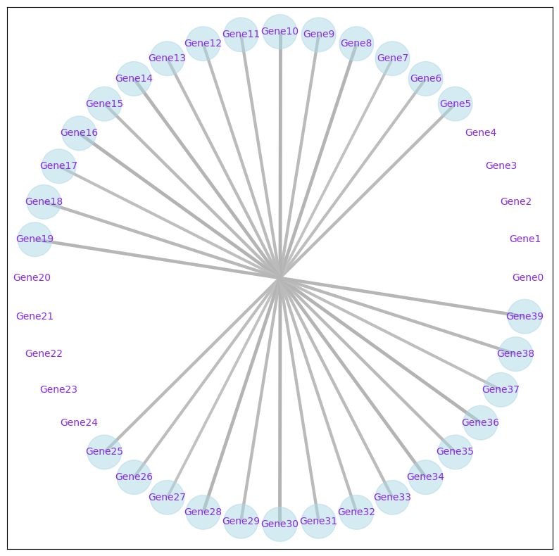
We use the draw_network_for_ddn function to visualize the network. For common networks, use mode="common". For differential networks, use mode="differential".

visualize.draw_network_for_ddn(common_net, nodes_non_isolated, node_size_scale=1, fig_size=10, mode='common', export_pdf=False)

<networkx.classes.graph.Graph at 0x22478c43bd0>

For more details about using DDN, as well aa choosing \(\lambda_1\) and \(\lambda_2\), check the next tutorials.